Dana Vrajitoru
B424 Parallel and Distributed Programming
Parallel Computer Graphics
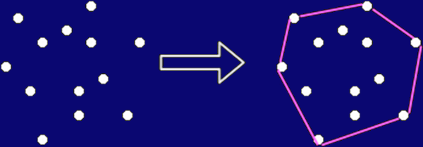
Convex Hull
- Given a number of points, find a subset of points forming a convex
polygon enclosing all the points.
- The points of the hull are called extreme points.
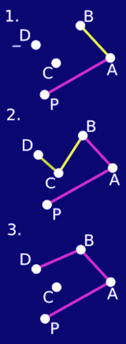
Graham's Scan
|
- Start with the lowest, left-most point.
- Order all the other points by angle with the first.
- Traverse the points from the bottom in order of the angle. For
each of them, if it's a left turn (1), accept it in the hull.
- If it's a right turn (2), discard the last point and connect the
new point with the one before the last (3). Then check backwards to
make sure the hull is convex.
- O(n log(n))
|
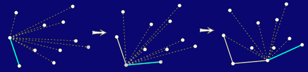
Jarvis's March
- Start similarly to Graham, with a left-most lowest point. Order
the others by angle with the first.
- Wrap around the points in counter-clockwise direction, starting
from the vertical down direction. The first encountered point is on
the hull.
- Start wrapping again from the new point with the first direction
being the line connecting it to the previous point.
- O(n*hull size), worst O(n2).
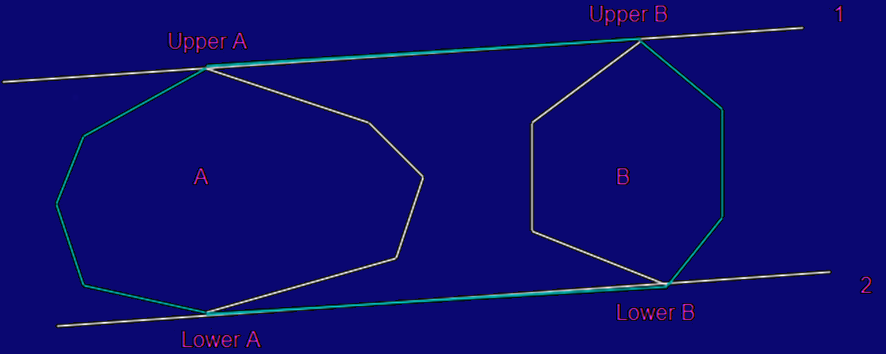
Parallel Version
- Divide the points in equal sets of points by the x coordinate.
- Compute the convex hull for each of them using some other
algorithm.
- Then combine the hull by connecting the lowest and highest points
from each of them, then remove the intermediate points.
Geometrical Transformations
- Translating - The coordinates of a two-dimensional object shifted by dx in the x-dimension and dy in the y-dimension are given by
x' = x + dx
y' = y + dy
- Scaling by factors Fx and Fy:
x' = x Fx
y' = y Fy
- Rotating by angle a around the origin:
x' = x cos(a) + y sin(a)
y' =-x sin(a) + y cos(a)
Partitioning into Processes
- The transformation can start from the target region and
go backward towards the source or the other way around.
- The division can be done in a grid or by rows.
Master() {
   for (i = 0, row = 0; i < 48; i++, row = row + 10)
      send(row, i); // send row no to each process
   for (i = 0; i < 480; i++) /* initialize temp */
      for (j = 0; j < 640; j++)
         temp_map[i][j] = 0;
   for (i = 0; i < (640 * 480); i++) { // for each pixel
      recv(oldrow,oldcol,newrow,newcol, any_source);
      if (!((newrow < 0)||(newrow >= 480)||
            (newcol < 0)||(newcol >= 640)))
         temp_map[newrow][newcol]=map[oldrow][oldcol];
   }
   for (i = 0; i < 480; i++) /* update bitmap */
      for (j = 0; j < 640; j++)
         map[i][j] = temp_map[i][j];
}
Slave() {
   recv(row, master); // receive row no.
   for (oldrow = row; oldrow < (row + 10);
        oldrow++)
      for (oldcol = 0; oldcol < 640; oldcol++)
      { // transform coords
          newrow = oldrow + delta_x; // shift
          newcol = oldcol + delta_y;
          send(oldrow,oldcol,newrow,newcol,
               master); // coords to master
      }
}
// In reverse order
Slave() {
   recv(row, master); // receive row no.
   for (newrow = row; newrow < (row + 10);
        newrow++)
      for (newcol = 0; newcol < 640; newcol++)
      { // transform coords
         oldrow = newrow / Fx; // reverse scale
         oldcol = newcol / Fy;
         send(oldrow,oldcol,newrow,newcol,
              master); // send coords to master
    }
}
Reversing the Rotation
- Basically, it's a rotate of -angle, knowing that sin(-a) = -sin(a)
cos(-a) = cos(a)
- oldrow = newrow*cos(a) - newcol*sin(a);
- oldcol = newrow*sin(a) + newcol*cos(a);
Mandelbrot Set
- Set of points in a complex plane that are quasi-stable (will
increase and decrease, but not exceed some limit) when computed by
iterating the function
zk+1 = zk2 + c
where zk+1 is the (k+1)th iteration of the complex
number
z = a + bi
and c is a complex number giving the position of the point in the
complex plane. The initial value for z is zero.
- The iterations are continued until magnitude of z is greater than
2 or the number of iterations reaches some arbitrary limit.
- For each point in the image, we start from c = x + i y, the
coordinates, and z=0+0i, (can be scaled by a factor). The amplitude is
sqrt(x2+y2).
z2 = a2 + 2abi + bi2 =
(a2 - b2) + (2ab)i
zreal = zreal2-zimag2+creal
zimag = 2 zreal zimag + cimag
- The number of iterations necessary for
zreal2+zimag2 >= 4 (or a given max) gives us the
color/shade of the pixel: 0 = white, max = black.
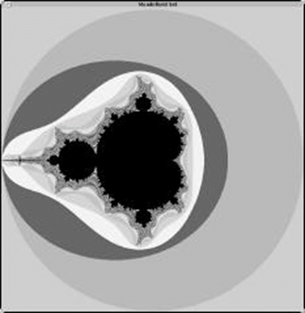
Range of the image: [-2, 2]x[-2, 2].
// Calculates the number of iterations
// for a pixel with creal = x, cimag = y.

int cal_pixel(float creal, float cimag) {
   int count=0, max = 256;
   float temp, lengthsq, zreal=0, zimag=0;
   do {
      temp = zreal*zreal - zimag*zimag + creal;
      zimag = 2*zreal*zimag + cimag;
      zreal = temp;
      lengthsq = zreal*zreal + zimag*zimag;
      count++;
   } while ((lengthsq < 4.0) && (count < max));
   return count;
}

Generate_fractal(int width, int height,
        float real_min, float real_max,
        float imag_min, float img_max) {
  // scale the fractal to the image size
   float scalex = (real_max - real_min)/width;
   float scaley = (imag_max - imag_min)/height;
   // generate the fractal:
   for (x = 0; x < width; x++)
      for (y = 0; y < height; y++) {
         creal = real_min + (float) x * scalex;
         cimag = imag_min + (float) y * scaley;
         color = cal_pixel(creal, cimag);
         display(x, y, color);
     }
}
Parallel Mandelbrot
- It is almost embarrassingly parallel.
- It depends on the access of each process to the display or the
stored image.
- Problem division: the calculation of the number of iterations for
each pixel can vary quite a lot.
- In general it is more suited for the pool of tasks division.
Master(min_real, max_real, min_imag, max_imag) {
   float scalex = (real_max - real_min)/width;
   float scaley = (imag_max - imag_min)/height;

   bcast([width,height,scalex,scaley,min_real,
         max_real,min_imag,max_imag]);

   for (i=0, row=0; i<48; i++, row += 10)
      send(row, i); // send row no. to process i
   for (i=0; i<(480 * 640); i++) {
      recv([x, y, color], any_source);
      display(x, y, color);
  }
}
Slave () {
   bcast([width,height,scalex,scaley,min_real,
         max_real,min_imag,max_imag]);
   recv(row, master);
   for (x = 0; x < width; x++)
      for (y = row; y < (row + 10); y++) {
         creal = real_min + (float) x * scalex;
         cimag = imag_min + (float) y * scaley;
         color = cal_pixel(creal, cimag);
         send([x, y, color], 0); //send to master
      }
}
Flood Fill
- Starting from a pixel in the image, fill the entire area that is
connected to it with a new color.
- We define the connectivity for (x, y) based on 4 neighbors: (x-1,
y), (x+1, y) (x, y-1), (x, y+1).
- The method is highly recursive. It scans the row containing the
pixel and as long as the color is contiguous, it calls itself
recursively on the pixel above and below.
- Hard to determine from the start how many recursive calls will
happen.
- Decomposition: exploratory and recursive.
- Probably easier in shared memory mode.
FloodFill (x0, y0, fill_color, original_color) {
   int color, x, y;
   x = x0; y = y0;
   getPixel(x, y, color);
   if (color == original_color) {
      while (color == original_color) {
         setPixel(x, y, fill_color);
         FloodFill(x, y+1, fill_color, original_color);
         FloodFill(x, y-1, fill_color, original_color);
         x = x - 1; // go left
         getPixel(x, y, color);
      }
      x = x0 + 1; y = y0;
      getPixel(x, y, color);
      while (color == original_color) {
         setPixel(x, y, fill_color);
         FloodFill(x, y+1, fill_color, original_color);
         FloodFill(x, y-1, fill_color, original_color);
         x = x + 1; // go right
         getPixel(x, y, color);
      }
   }
}
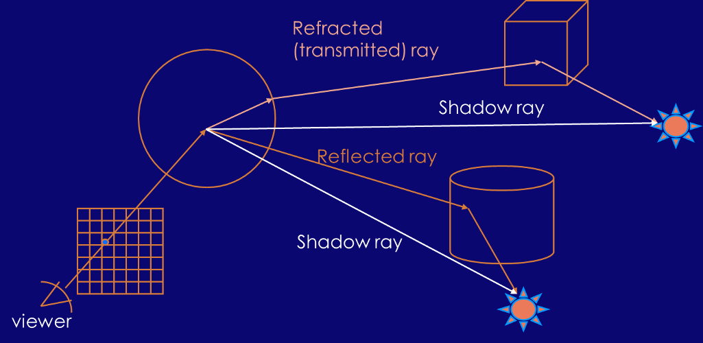
Ray Tracing - the Method
- Send a ray from each pixel to the reverse direction of the light
coming in.
- Compute the closest intersection of this ray with any object.
- Consider the ray in the direction of each light source from the
intersection point (shadow rays).
- For each of them, check if the ray intersects another object or
not. Compute the local contribution from the rays without
intersection.
- Add to this the light obtained by reflection and refraction in
this point computed recursively.
Speed-up Techniques
- Recursive depth limit.
- Bounding boxes or spheres reduce the intersection calculation.
- Vista buffer: projecting the objects onto the screen in
pre-processing so we know what regions are empty.
- Light projection on a cube around each object in pre-processing.
Parallel Ray Tracing
- The image can be divided equally into pieces (rectangles, rows,
pixels) assigned to each process.
- The computation of each pixel is quite intensive and can vary
based on the number of objects intersecting the ray.
- Also suitable for pool of tasks.
- 2008: Intel on 4 quad-core Xeon CPUs, running Quake Wars at
15-20fps. GPU-based implementations: Nvidia: programmable Ray Tracing
Engine OPTIX (2009).
- Currently: Intel using cloud computing and the Intel Many
Integrated Core (MIC) architecture. Reported 38fps in HD.
Existing Techniques
- Screen subdivision: dividing the pixels to be computed among the
processes. Load balancing issues.
- Object subdivision: geometrical distribution of objects to
processes. The processes need to exchange rays.
- Functional decomposition: assigning different task, such as
"reflective rays computation" or "shadow ray" computations to each
process. Can be implemented in a client-server model.